Scatterplots and Correlation: How Your Choices Pair Up Without You Noticing

Introduction: The Unseen Connections

Think about your day. Did the number of coffees you drank seem to connect with how jittery you felt? Does the time you spend exercising pair up with how well you sleep? Maybe you've noticed that longer study sessions tend to result in better test scores? Your life is full of these connections, subtle pairings between choices, actions, and outcomes, often happening without you consciously noticing.

Humans are pattern-seeking creatures. We instinctively look for connections to make sense of the world, like whether more study time relates to higher grades, or if there's a link between a house's size and its price. But are those connections real, or just a coincidence? Statistics gives us the tools to move from a simple hunch to a more objective understanding.

So far, you've read about describing single pieces of information: the typical value (like the mean or median), how spread out things are (standard deviation), and the overall shape of the data (like the bell curve). That's crucial groundwork, but the truly interesting, juicy stories often lie in how different pieces of information relate to each other.

This is a big step. We're moving from univariate data (analysing one variable at a time) to bivariate data (analysing two). This leap is where data science starts to get really powerful, as it allows us to build models and make predictions.

This article moves you into exploring these relationships. You'll learn how to visualise these pairings using a simple graph called a scatterplot, how to measure the strength of a straight-line connection with a number called correlation, and even how to make basic predictions. It’s about looking beyond individual facts and starting to see the patterns that connect them, revealing how your choices might be pairing up in ways you hadn't realised. For now, you'll be focusing only on relationships between two quantitative variables (things you can measure numerically).

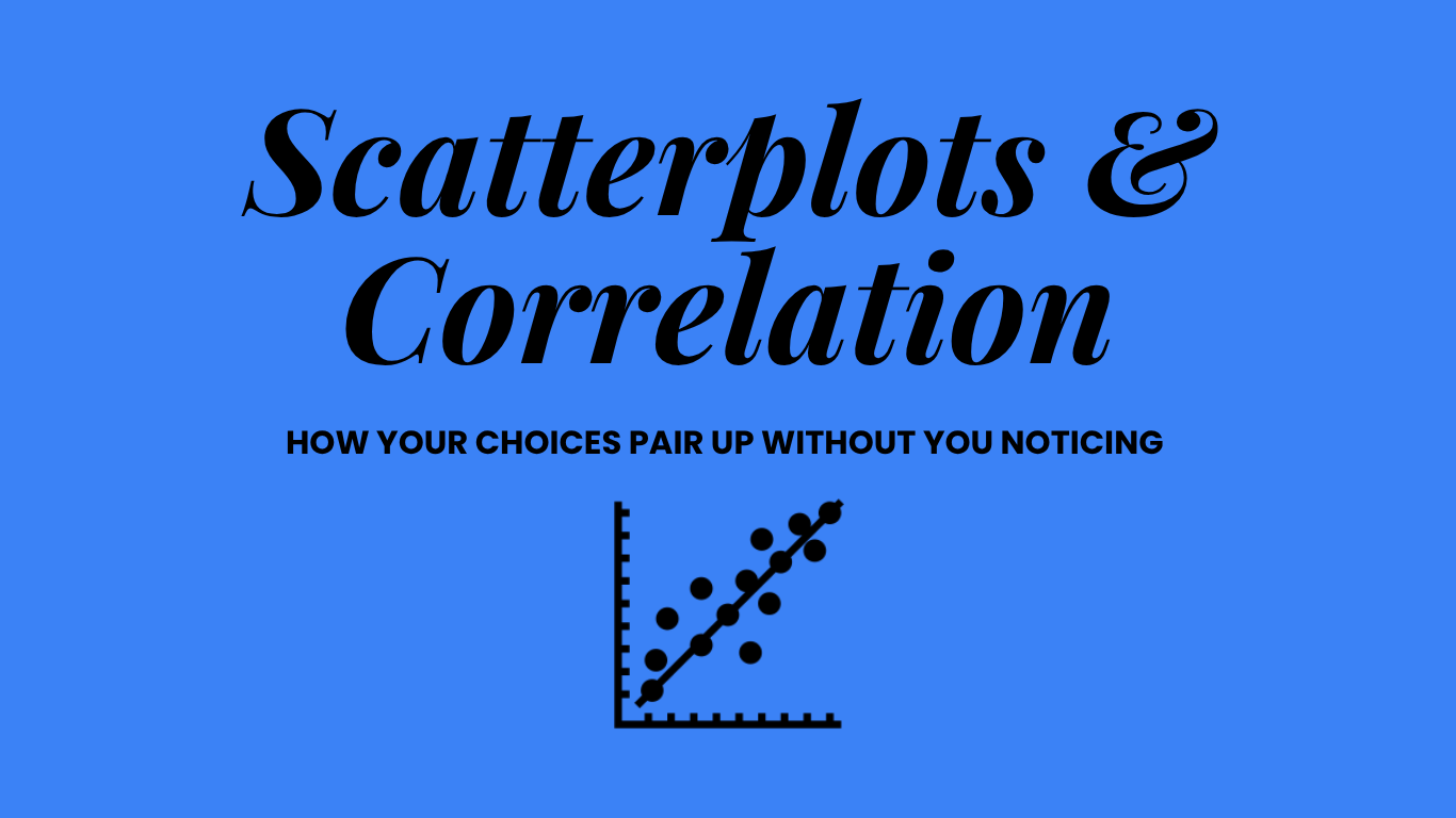
Visualising Relationships: The Scatterplot

Before jumping into complex calculations, the first step is always to look at your data. When you want to see how two quantitative variables might be related, the best tool is the scatterplot. It's a simple, powerful graph that forms the foundation of this entire topic. Imagine you have data on several students, including how many hours they studied ($x$) and their exam score ($y$). A scatterplot simply puts a dot on a graph for each student, positioned according to their study hours (horizontally) and their score (vertically).

Explanatory vs. Response Variables

When creating a scatterplot, you usually have an idea about which variable might influence the other. The variable you think is doing the influencing is called the explanatory variable (or independent variable) and it goes on the x-axis (horizontal). The variable you think is being affected is the response variable (or dependent variable) and it goes on the y-axis (vertical). In the study hours vs. exam score example, study hours explain the score, so hours go on the x-axis and score goes on the y-axis.

Sometimes, the choice is obvious. If you're comparing rainfall and crop yield, rainfall explains the yield, not the other way around. Other times, it might not be clear. If you're comparing a student's SAT score in Maths and English, which one explains the other? In that case, the choice might be arbitrary, and you're just looking for an association, not a causal link.

How to Describe a Scatterplot: Look for the Obvious

Looking at the cloud of points isn't enough; you need a systematic way to describe what you see. To properly analyse a scatterplot, you should always comment on these four features:

• Direction: Does the cloud of points generally drift upwards or downwards as you look from left to right?
  • Positive Association: Points drift upwards. As the x-variable increases, the y-variable tends to increase too (e.g., more study hours, higher score).
  • Negative Association: Points drift downwards. As the x-variable increases, the y-variable tends to decrease (e.g., more time spent gaming, lower score).
• Form: Does the pattern look roughly like a straight line (linear), or does it follow a curve (e.g., a 'U' shape or an 'S' shape)? Sometimes you might see distinct groups or clusters, or maybe there's no clear pattern at all.
• Strength: How tightly do the points follow the pattern?
  • Strong: Points are very close to a clear line or curve. You could easily draw a line through them.
  • Moderate: Points follow the general trend but are more spread out. A "fat pencil" might cover them.
  • Weak: Points are very scattered, and the trend is barely visible. It's just a vague cloud.
• Outliers: Are there any points that fall far away from the overall pattern? These individuals might be unusual cases (e.g., a student who studied for 0 hours but got a 90) and can sometimes strongly influence your conclusions.

It's crucial to comment on all four of these features every time you see a scatterplot. Skipping one can lead to a completely wrong conclusion. For example, you might see a strong pattern (Strength) that is curved (Form), but if you only describe it as 'strong', you might later try to fit a straight line, which would be totally inappropriate!

Quantifying Linear Relationships: Correlation ($r$)

Looking at a scatterplot gives you a feel for the relationship, but "moderate negative" isn't very precise. What's 'moderate' to you might be 'weak' to someone else. You need a number, an objective measure, to quantify the direction and strength of the linear association between two quantitative variables. This number is the correlation coefficient, usually just called correlation and written as $r$.

It's important to know that the $r$ value we're talking about is technically the Pearson correlation coefficient. It's the most common one, but not the only one. It's designed to be a number that backs up what your eyes see... if what your eyes see is a straight line.

Think of $r$ as a numerical summary of a linear pattern in a scatterplot. Here are its key properties:

• Range: $r$ is always between -1 and +1, inclusive. You will never get an $r$ of 2 or -3.
• Direction:
  • $r > 0$ indicates a positive association (points trend upwards).
  • $r < 0$ indicates a negative association (points trend downwards).
• Strength:
  • $r$ close to +1 or -1 means the points lie very close to a straight line (a strong linear relationship). $r = 1$ or $r = -1$ means a perfect straight line.
  • $r$ close to 0 means there is a very weak linear relationship (the points are scattered with no clear line).
• Linearity Only: This is a big one. Correlation $r$ only measures the strength and direction of a straight-line relationship. You could have a perfect, U-shaped curve where the points form a beautiful parabola, but the $r$ value could be 0 or very close to it. This is because, for the first half of the 'U', the association is negative, and for the second half, it's positive. They can cancel each other out! This is why you must always look at the scatterplot first. Never, ever report an $r$ value without having seen the graph.
• No Units: Correlation is a pure number. It doesn't change if you measure height in inches or centimetres. The correlation between height and weight is the same, regardless of units.
• Symmetry: The correlation between variable X and variable Y is the same as the correlation between Y and X. It doesn't care which you call 'explanatory'.
• Sensitivity to Outliers: Just like the mean, the correlation $r$ can be significantly changed (or "pulled") by one or two extreme outliers. A single point far from the main cloud can dramatically strengthen or weaken your $r$ value.

Correlation tells you how well your data points hug a straight line. It doesn't care about curves!

The Crucial Caveat: Correlation vs. Causation

This might be the single most important warning you'll ever hear in statistics: correlation does not imply causation. Just because two variables tend to pair up, moving together in a predictable way, doesn't automatically mean one is causing the other to change.

This is the most repeated phrase in all of statistics, and for good reason. It's so tempting to see a strong $r$ value, like +0.9, and shout 'A causes B!' But the world is far more complicated than that.

Think back to the ice cream sales and crime rates example. They are strongly positively correlated – when one goes up, the other tends to go up. But concluding that ice cream causes crime would be absurd. There's a hidden, or lurking variable, at play: temperature. Hot weather drives up both ice cream sales and the number of people outdoors (increasing opportunities for crime). Temperature is causing changes in both variables, creating the illusion of a direct link between them.

Another example: there's a positive correlation between the number of firefighters at a fire and the amount of damage done. Does this mean firefighters cause damage? No! The lurking variable is the size of the fire. Bigger fires attract more firefighters and cause more damage.

This is called a confounding relationship. The lurking variable (size of the fire) is confounded with the explanatory variable (number of firefighters). Because they both rise together, you can't tell which one is actually responsible for the damage. The only reliable way to break this link and prove causation is to run a controlled experiment where you, for example, randomly assign different numbers of firefighters to identical fires... which is obviously absurd and unethical. In many real-world scenarios, experiments aren't possible, so we have to be very, very careful about claiming causation from correlation alone.

Spotting a correlation is often the start of an investigation, not the end. It suggests a potential connection, but you need more evidence, usually from carefully designed experiments that control for lurking variables, to establish a cause-and-effect relationship.

Introduction to Prediction: Linear Regression

Okay, so you've looked at your scatterplot, confirmed the relationship looks reasonably linear, and calculated the correlation $r$ to check its strength. If the linear pattern is strong enough, you might want to do more than just describe it – you might want to use it to make predictions. This is where linear regression comes in.

Think of it as drawing a 'line of best fit' through the cloud of points. But 'best' needs a proper mathematical definition.

The goal is to find the one straight line that best captures the trend in your scatterplot. This special line is called the least-squares regression line (LSRL). It gets its name because it's calculated to minimise the sum of the squared vertical distances (called residuals) between each data point and the line itself. Imagine drawing vertical lines from each point to your regression line; the LSRL is the one line that makes the total area of squares built on those vertical lines as small as possible.

Why are the distances squared? Two main reasons. First, it gets rid of negative and positive residuals (points above and below the line) so they don't just cancel each other out. Second, it heavily penalises points that are very far away from the line. This means the line will be 'pulled' quite strongly towards any significant outliers, which is another reason why identifying outliers is so important.

The equation of the LSRL will look familiar if you remember your algebra:

$\hat{y} = a + bx$

• $\hat{y}$ (read "y-hat") is the predicted value of the response variable for a specific value of $x$. It's not the actual value, but the value the line predicts.
• $x$ is the value of your explanatory variable you're plugging in.
• $b$ is the slope. This is often the most interesting part. It tells you, on average, how much you expect $\hat{y}$ to change for every one-unit increase in $x$. For example, if $b=5$ in the study hours ($x$) vs. exam score ($y$) example, it means you predict the score to increase by 5 points for each additional hour studied. The slope is the engine of your model. It's the numerical value of the relationship. A positive $b$ means a positive association, and a negative $b$ means a negative one. A $b$ of 0 would mean the line is flat, and there's no linear relationship between $x$ and $y$ at all.
• $a$ is the y-intercept. This is the predicted value of $\hat{y}$ when $x$ is exactly 0. You need to be careful interpreting this! If $x=0$ doesn't make sense in the context of your data (like 0 study hours, or 0 height), or if your data doesn't include values near $x=0$, the intercept might just be a mathematical necessity for the line, not a meaningful prediction. For example, in a model predicting weight ($y$) from height ($x$), the y-intercept would be the predicted weight for a person with zero height. This is biologically impossible and nonsensical. In this case, the intercept is just a mathematical anchor for the line within the range of your data and has no useful real-world interpretation.

The Danger of Extrapolation

It's tempting to use your shiny new regression line to predict far beyond the range of your original data. Don't do it! This is called extrapolation. You have no evidence that the linear relationship continues outside the range you observed. Maybe the pattern curves off, flattens out, or does something completely different. A model that predicts study scores might be linear from 1-10 hours, but it probably flattens out after 20 hours (you can't get a score of 200). Stick to making predictions for x-values that are within or very close to the range of your data (interpolation).

Conclusion: Uncovering the Hidden Pairings

You've added some powerful tools to your statistical toolkit! You've moved from simply describing data to actively modelling it. You can now look beyond single variables to see how pairs of quantitative variables might be related using scatterplots. You can describe the direction, form, and strength of these relationships visually, and quantify the linear component using the correlation coefficient, $r$. You've also taken your first step into modelling by learning about the least-squares regression line for making predictions.

Crucially, you've also learned the essential caution: seeing a pairing, even a strong one, doesn't mean you've found a cause. Correlation is a clue, an invitation to investigate further, but it's rarely the final answer on its own. It's the beginning of a question, not the end of the answer.

So, you can describe relationships in the data you have. But how much can you trust these patterns? Could a correlation you see in your small sample just be a random fluke? To answer that, you need to understand the rules of chance. The next step in your journey is to dive into the world of probability and sampling distributions – the foundations you need to start making reliable inferences about the bigger picture. That's the bridge from Descriptive Statistics (describing what you have) to Inferential Statistics (using what you have to make educated guesses about what you don't), and it's where the real magic happens.