The Problem: We Never Have the Whole Picture
In our last post, we looked at probability distributions—the "God's eye view" of the world. If you know exactly how a coin behaves, or exactly the average height of every human on earth, you can predict outcomes perfectly.
But here is the harsh reality of data science: We almost never have the population data.
We don't know the true average income of a country. We don't know the true effectiveness of a new drug on every human. We only have a sample: a small slice of reality.
So, we have a massive problem. How can we possibly say anything confident about the "Population Truth" (the parameter, $\mu$) when all we have is a "Sample Guess" (the statistic, $\bar{x}$)? What if our sample is weird? What if we just got lucky (or unlucky)?
The answer lies in one of the most beautiful, almost magical concepts in mathematics: The Central Limit Theorem.
What is a Sampling Distribution?
To understand the magic, we have to perform a mental experiment. Imagine you want to know the average height of people in your city.
- You go out and survey 30 random people. You calculate their average height ($\bar{x}_1$). Maybe it's 170cm.
- You go out again and survey a different 30 people. You calculate their average ($\bar{x}_2$). Maybe it's 168cm.
- You do this again. And again. And again. 1,000 times.
You now have 1,000 different "averages." If you were to plot all these averages on a histogram, you would have created a Sampling Distribution.
A Sampling Distribution is not a distribution of people. It is a distribution of samples. It tells us how much our sample means tend to vary from the true population mean.
The Central Limit Theorem (CLT)
Here is where it gets wild. In the real world, data is often messy. Income data is heavily skewed (mostly low, some super high). Dice rolls are uniform (flat). Customer wait times are exponential.
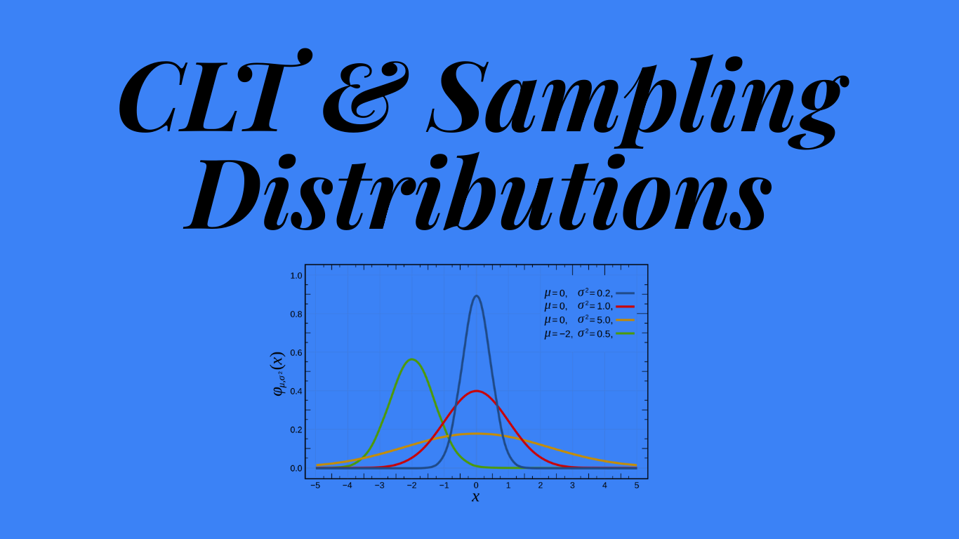
The Central Limit Theorem (CLT) states that if you take large enough samples ($n \ge 30$ is the rule of thumb) from a population, the sampling distribution of the sample means will always be Normally Distributed (a bell curve), even if the original population is not!
Think about that. You can start with a chaotic, skewed, or flat population. But if you gather enough data and take averages, order emerges from the chaos. The averages will form a perfect bell curve centered on the true population mean.
CLT Simulator: Order from Chaos
Choose a "Parent Population" shape (Uniform or Skewed). Then, increase the Sample Size ($n$). Watch how the distribution of Means (bottom chart) turns into a Bell Curve, regardless of the starting shape.
Standard Error: Shrinking the Spread
The CLT tells us the shape (Normal) and the center (True Mean). But what about the spread? How "wide" is our bell curve of sample means?
This spread is called the Standard Error (SE). It is different from Standard Deviation. Standard Deviation measures how different people are. Standard Error measures how different samples are.
The formula for Standard Error is:
$$SE = \frac{\sigma}{\sqrt{n}}$$
Where $\sigma$ is the population standard deviation and $n$ is the sample size.
Look at the denominator ($\sqrt{n}$). This proves the Law of Large Numbers: As your sample size ($n$) gets bigger, your Standard Error gets smaller. The bell curve gets narrower and taller. This means your sample means are getting closer and closer to the true population mean.
Visualizing Standard Error
The grey curve is the population (spread of individuals). The blue curve is the sampling distribution (spread of averages). Drag the slider to increase sample size ($n$) and see the error shrink.
Why This Matters: The Key to Inference
Why do we care about imaginary distributions of samples we never took? Because knowing that sample means follow a Normal Distribution allows us to calculate Probability.
If we take a sample and get a result that is way out on the "tail" of the Sampling Distribution, we know that such a result is extremely rare if chance were the only factor. This is the logic behind Hypothesis Testing.
- We can calculate Confidence Intervals: "We are 95% confident the true mean is between X and Y."
- We can calculate P-Values: "The probability of seeing this result by luck is only 1%."
Without the Central Limit Theorem, we couldn't trust our samples. With it, we can bridge the gap between the small data we have and the big truth we seek.
Now that we know how samples behave, we are ready for the main event. How do we scientifically prove something is true? Join us next time for Hypothesis Testing & The P-Value.


